
FIR filter overview
When we implement an FIR filter in FPGA or ASIC the major cost in terms of area resources derives from the multiplier units required for coefficient multiplication. Depending on the frequency response of the filter, the number of coefficients (or filter taps) could become large.
As is clear from the FIR filter architecture in Figure 1, the number of multiplier operations is equal to the number of taps. For a long filter, the area required will be demanding.
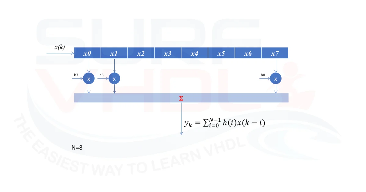
Figure 1 – Classic FIR architecture
FIR architecture possible optimization
For applications where the sampling speed is low, or where the ratio between the system clock and the filter output speed is high, we can adopt a resource sharing strategy.
Another optimization possibility can be adopted when the coefficients of the filter can be expressed as powers-of-two. In this case, the multiplication can be performed with shift-and-add operations.
If you need to refresh the FIR architecture you can take a look at this post: https://surf-vhdl.com/how-to-implement-fir-filter-in-vhdl/
Here we want to address a very interesting FIR architecture optimization that we can adopt when we can take advantage of some hypothesis on input data.
Shaping filter for modulator system
In this post, we talk about the implementation of an ASK modulator: https://surf-vhdl.com/implement-digital-ask-modulator-vhdl/
In the modulator, the output shaping filter could be very demanding in terms of area, but an optimization could be implemented.
If the modulation is a quadrature modulation such as ASK, BPSK, QPSK, the input symbols to the matching output filter will be of this form:
- +A
- –A
where A is the amplitude of the modulated signal.
In this case, we can set A=1, so the input symbols to the output matched filter will be +/-1.
Just to clarify, Figure 2 shows an example of QPSK modulation where the amplitude of in-phase and quadrature channel is +/-1:
- “00” I=+1, Q=+1
- “01” I=-1, Q=+1
- “11” I=-1, Q=-1
- “10” I=1, Q=-1
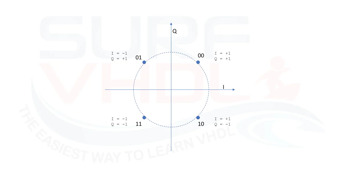
Figure 2 – QPSK modulation example
In this case, the input pipe to the filter will always contain +/-1.
As a first optimization, the multipliers can be replaced with a sign change of the coefficient.
This is a good starting optimization, but in this post we want to go further.
Let’s optimize our filter even more.
Implementing the memory mapped filter architecture
As said before, the input filter pipe will get the +/-1 as the input value.
We can encode:
- +1 => ‘0’
- -1 => ‘1’
For the sake of simplicity, let the filter length be just 4 taps. For an input filter pipe of 4, let’s see what the input filter pipe looks like for all possible input patterns in Figure 3
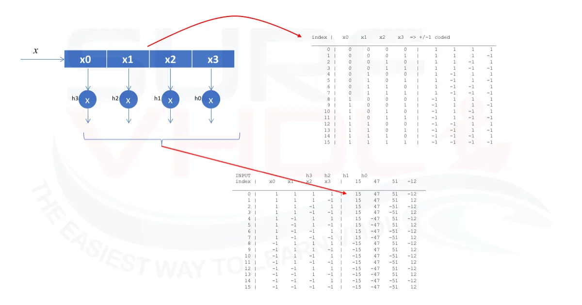
 index |   x0    x1    x2    x3  => +/-1 coded
____________________________________________________________
     0 |    0     0     0     0   |     1     1     1     1
     1 |    0     0     0     1   |     1     1     1    -1
     2 |    0     0     1     0   |     1     1    -1     1
     3 |    0     0     1     1   |     1     1    -1    -1
     4 |    0     1     0     0   |     1    -1     1     1
     5 |    0     1     0     1   |     1    -1     1    -1
     6 |    0     1     1     0   |     1    -1    -1     1
     7 |    0     1     1     1   |     1    -1    -1    -1
     8 |    1     0     0     0   |    -1     1     1     1
     9 |    1     0     0     1   |    -1     1     1    -1
    10 |    1     0     1     0   |    -1     1    -1     1
    11 |    1     0     1     1   |    -1     1    -1    -1
    12 |    1     1     0     0   |    -1    -1     1     1
    13 |    1     1     0     1   |    -1    -1     1    -1
    14 |    1     1     1     0   |    -1    -1    -1     1
    15 |    1     1     1     1   |    -1    -1    -1    -1
Can you guess what the next step could be?
Right! A Look-Up-Table
for any input pattern, we can use the input filter pipeline as the address of a LUT that contains the output filter value.
                 INPUT                   Impulse response
 index |    x0    x1    x2    x3   |    15    47    51   -12    |  sum(h*x)
__________________________________________________________________________
     0 |      1     1     1     1  |    15    47    51   -12    |    101
     1 |      1     1     1    -1  |    15    47    51    12    |    125
     2 |      1     1    -1     1  |    15    47   -51   -12    |     -1
     3 |      1     1    -1    -1  |    15    47   -51    12    |     23
     4 |      1    -1     1     1  |    15   -47    51   -12    |      7
     5 |      1    -1     1    -1  |    15   -47    51    12    |     31
     6 |      1    -1    -1     1  |    15   -47   -51   -12    |    -95
     7 |      1    -1    -1    -1  |    15   -47   -51    12    |    -71
     8 |     -1     1     1     1  |   -15    47    51   -12    |     71
     9 |     -1     1     1    -1  |   -15    47    51    12    |     95
    10 |     -1     1    -1     1  |   -15    47   -51   -12    |    -31
    11 |     -1     1    -1    -1  |   -15    47   -51    12    |     -7
    12 |     -1    -1     1     1  |   -15   -47    51   -12    |    -23
    13 |     -1    -1     1    -1  |   -15   -47    51    12    |      1
    14 |     -1    -1    -1     1  |   -15   -47   -51   -12    |   -125
    15 |     -1    -1    -1    -1  |   -15   -47   -51    12    |   -101
As you can see, the filter implementation is reduced to a 1-bit shift register and a LUT.
We could not ask for more!
Of course, there is a problem. As is clear, the LUT dimension will depend on the filter length in an exponential way:
- filter length =3 => LUT length = 8
- filter length =4 => LUT length = 16
- filter length =N => LUT length = 2^N
for a 16-tap filter, we get 2^16 = 65536 (64K) LUT length.
It is a big deal!
But we can do some optimization even in this case.
Let’s see what happens if the filter length is 8 as in Figure 4
In this case, the LUT length will be 2^8 = 256
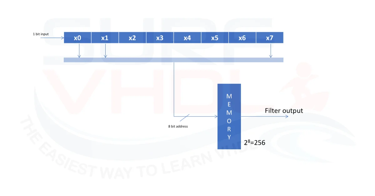
Figure 4 – FIR 8 taps single LUT of 256 entries
We can rearrange the filter architecture as in Figure 5. Instead of using the entire filter pipe of 8 bit, we can break into 2×4 bit pipe and add the output of the LUT.
This is very similar to the classical filter architecture that you can see here: https://surf-vhdl.com/how-to-implement-fir-filter-in-vhdl/
The result is that the filter LUT is no more 256, but 2 x16.
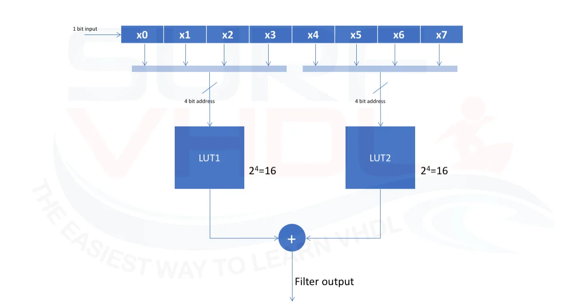
Figure 5 – FIR 8 taps using 2 LUT of 16 entries
More generally, if we need a filter length of N, we can implement the same filter using two LUTs of dimension 2^(N/2)
in the case of 8, we have 2 x 2^4=16 instead of 2^8=256,
I think it could be a good optimization.
Filter LUT implementation
In the previous section, we addressed how to optimize a matched filter architecture for an ASK modulator. Now we will understand how to compute the LUT value starting from a given filter impulse response.
We will use Matlab/Octave code to compute the LUT coefficient.
The first thing we need is the filter input pattern as the binary vector that we will use as LUT address.
Now we remap this 0/1 vector as +/-1 where
- 0=> +1
- 1=>-1
this coding will give the 2’s complement encoding for free.
In fact, in 2’s complement representation (see the post: https://surf-vhdl.com/binary-number-representation/) the MSB is the sign of the number
- ‘0’ => positive or zero
- ‘1’ => negative
Using this coding pattern, the input to the filter will be the MSB of the mapper. Of course, also the mapper will be simplified using only 1-bit coding.
Now that we get all the possible input pattern to the filter, let’s compute the LUT values for each LUT address.
If you remember the FIR filter equation
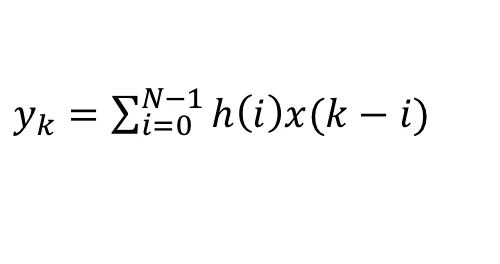
the LUT value can be computed as a simple matrix-vector multiplication where the input matrix xM represents all the possible values of the input pipe and h is the filter impulse response. Below is the Matlab/Octave script:
fileLen = 8;
% generate the address matrix
d = (0:2^fileLen-1)';
t = de2bi(d,[],2,'left-msb');
[d t]

% convert address matrix in +/-1
xM = 1-2*t

% filter coefficient
h = [15  47 51 -12]

% create the LUT for the filter
Lut = mtimes(xM,h')
Now we have all the information to implement the VHDL code for the filter.
VHDL implementation of a simplified Modulator filter
Here below you can find the VHDL implementation of the modulator filter implemented with LUT.
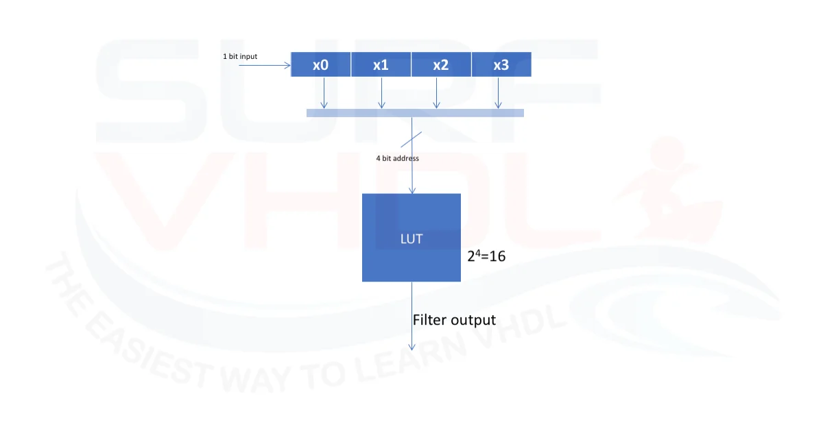
Figure 6 – FIR 4 taps LUT architecture
The filter is implemented as 4 taps filter. Here below a possible VHDL implementation for the FIR-LUT filter:
library ieee;
use ieee.std_logic_1164.all;
use ieee.numeric_std.all;

entity filter_lut4 is
port (
  i_clk          : in  std_logic;
  i_rstb         : in  std_logic;
  i_data_ena     : in  std_logic;
  i_data         : in  std_logic;  -- 1 bit input
  o_data_valid   : out std_logic;
  o_data         : out std_logic_vector(7 downto 0));
end filter_lut4;

architecture rtl of filter_lut4 is
constant C_FILTER_LEN            : integer := 4;
constant C_LUT_BIT               : integer := 8;
---------------------------------------------------------------------------------------------------
type t_lut is array (0 to (2**C_FILTER_LEN)-1) of integer range -(2**C_LUT_BIT) to (2**C_LUT_BIT)-1;

constant C_LUT                           : t_lut := (
   101 ,     125 ,    -1 ,    23 ,     7 ,    31 ,   -95 ,   -71 ,    71 ,    95 ,   -31 ,    -7 ,   -23 ,     1 ,  -125 ,  -101 );

signal r_data_pipe                         : std_logic_vector(C_FILTER_LEN-1 downto 0);
signal r_data_ena                          : std_logic;

begin

p_data : process(i_clk,i_rstb)
begin
  if(i_rstb='0') then
    r_data_pipe    <= (others=>'1');
    r_data_ena     <= '0';
    o_data         <= (others=>'0');
    o_data_valid   <= '0';
  elsif(rising_edge(i_clk)) then
    o_data_valid   <= r_data_ena;
    r_data_ena     <= i_data_ena;
    if(i_data_ena='1') then
      r_data_pipe    <= i_data&r_data_pipe(r_data_pipe'length-1 downto 1);
    end if;
    o_data         <= std_logic_vector(to_signed(C_LUT(to_integer(unsigned(r_data_pipe))),C_LUT_BIT));
  end if;
end process p_data;

end rtl;
In the next example, there is reported the VHDL implementation of an 8 taps filter cascading the two previous 4 taps filter as in Figure 5.
library ieee;
use ieee.std_logic_1164.all;
use ieee.numeric_std.all;

entity filter_lut4x2 is
port (
  i_clk          : in  std_logic;
  i_rstb         : in  std_logic;
  i_data_ena     : in  std_logic;
  i_data         : in  std_logic;  -- 1 bit input
  o_data_valid   : out std_logic;
  o_data         : out std_logic_vector(8 downto 0));
end filter_lut4x2;

architecture rtl of filter_lut4x2 is
constant C_FILTER_LEN            : integer := 4;
constant C_LUT_BIT               : integer := 8;
---------------------------------------------------------------------------------------------------
type t_lut is array (0 to (2**C_FILTER_LEN)-1) of integer range -(2**C_LUT_BIT) to (2**C_LUT_BIT)-1;

constant C_LUT1                           : t_lut := (
   101 ,     125 ,    -1 ,    23 ,     7 ,    31 ,   -95 ,   -71 ,    71 ,    95 ,   -31 ,    -7 ,   -23 ,     1 ,  -125 ,  -101 );
constant C_LUT2                           : t_lut := (
   -14 ,     138 ,    18 ,   170 ,  -122 ,    30 ,   -90 ,    62 ,   -62 ,    90 ,   -30 ,   122 ,  -170 ,   -18 ,  -138 ,    14 );

signal r_data_pipe1                         : std_logic_vector(C_FILTER_LEN-1 downto 0);
signal r_data_pipe2                         : std_logic_vector(C_FILTER_LEN-1 downto 0);
signal r_data_ena                           : std_logic;

signal w_addr_lut1                          : integer range 0 to ((2**C_FILTER_LEN)-1);
signal w_addr_lut2                          : integer range 0 to ((2**C_FILTER_LEN)-1);

begin
w_addr_lut1     <= to_integer(unsigned(r_data_pipe1));
w_addr_lut2     <= to_integer(unsigned(r_data_pipe2));

p_data : process(i_clk,i_rstb)
begin
  if(i_rstb='0') then
    r_data_pipe1   <= (others=>'1');
    r_data_pipe2   <= (others=>'1');
    r_data_ena     <= '0';
    o_data         <= (others=>'0');
    o_data_valid   <= '0';
  elsif(rising_edge(i_clk)) then
    o_data_valid   <= r_data_ena;
    r_data_ena     <= i_data_ena;
    if(i_data_ena='1') then
      r_data_pipe1    <= i_data&r_data_pipe1(r_data_pipe1'length-1 downto 1);
      r_data_pipe2    <= r_data_pipe1(0)&r_data_pipe2(r_data_pipe2'length-1 downto 1);
    end if;
    o_data         <= std_logic_vector(to_signed(C_LUT1(w_addr_lut1),o_data'length) + to_signed(C_LUT2(w_addr_lut2),o_data'length));
  end if;
end process p_data;

end rtl;
Notice that the output filter dynamics depend on how many bits we quantize the filter coefficients. In this post, we did not address the filter design and quantization.
An example of FIR filter coefficient quantization is given in this post: https://surf-vhdl.com/how-to-quantize-fir-coefficient/
Simulation of filter VHDL code
Figure 7 presents the simulation of the 8-tap FIR filter output in Figure 5 compared with the reference generated using Matlab/Octave code below.
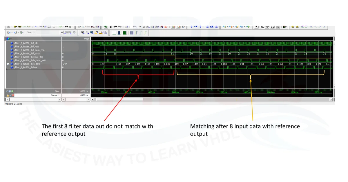
Figure 7 – ModelSim VHDL simulation for FIR 8 taps using 2 LUT of 16 entries
As is clear in the transient part, i.e. when the number of input data is less than the filter length, there is a mismatch between the reference output and VHDL output. In this simulation the filter length is 8 symbols, so the mismatch can be at least 8 output filtered symbols. In order to facilitate the check of the filter matching, there is an “error_flag” in yellow.
Notice that if we want to match all the filter output, we need to initialize the Matlab filter as the VHDL implementation filter.
Layout of VHDL simplified matching filter
Figure 8 reports the RTL view of the 8-tap filter described in the previous paragraph. As is clear, the filter structure is very straightforward. The layout shows that the area resources use very few cells. The same filter implemented using the classical architecture is much more demanding.
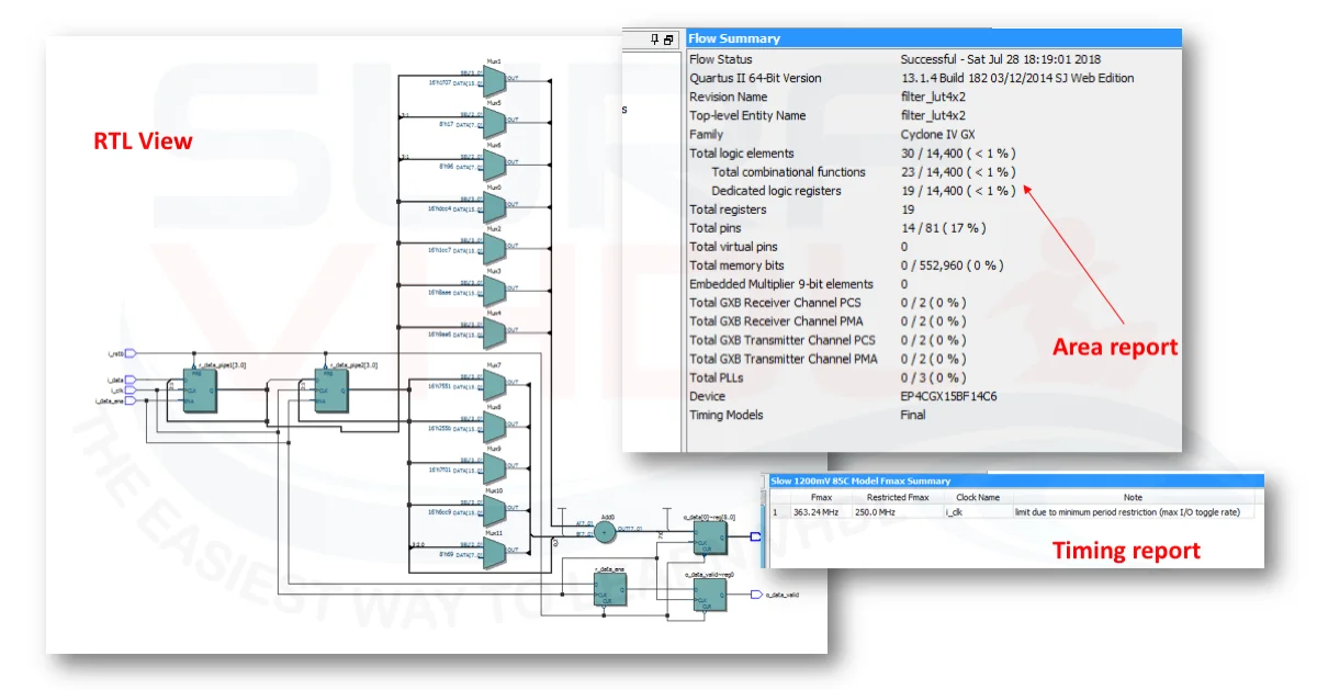
Figure 8 – Quartus II Layout for VHDL implementation of FIR 8 taps using 2 LUT of 16 entries
Conclusion
In this post, we addressed the VHDL implementation of a digital filter using a LUT approach.
This filter architecture is very efficient in terms of area and timing resources.
Like all good things, this architecture has the drawback that the input data can be only +/-1.
Even with this restriction, we can use this optimization in a wide modulator filter implementation if the modulation can be expressed as an amplitude-like modulation.
An example was given for a QPSK modulation.
References
[2] https://www.mathworks.com/
[4] https://www.gnu.org/software/octave/
[5] “DSP Architecture Design Essentials”, Authors: Marković, Dejan, Brodersen, Robert W.