

A moving average is a signal processing technique that smooths out short-term fluctuations and highlights longer-term trends in data. It is widely used in digital systems for noise reduction, decimation filtering, and data smoothing. In FPGA designs, implementing an efficient moving average requires careful hardware architecture to minimize resource usage while maintaining throughput.
In some applications, we need to perform a moving average on the input data of our design.
In the moving average, for each incoming sample, we need to compute an equation like:
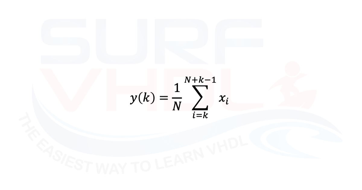
Moving average equation
For N=4:
y(0) = 1/4 (x0+x1+x2+x3)
y(1) = 1/4 (x1+x2+x3+x4)
At the moment, leave the 1/4 apart and focus on the add section.
y(2) = (x2+x3+x4+x5)
in other words,
y(2) = y(1) + x5 - x1
| Step | xn | xn-1 | xn-2 | xn-3 | Acc | Output |
|---|
This consideration can simplify the architecture of the moving average block using a simple accumulator, adding the incoming sample and subtracting the outgoing one, as in Figure 2:
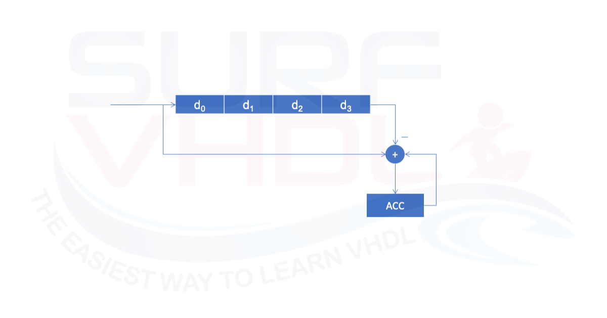
Figure 2 – Moving average architecture for N=4
The division by N becomes very simple when N is a power of two. In fact, in this case, the division is performed simply as a right shift.
When N is not a power of two you can refer to this post where you can learn how to implement a division by constant.
VHDL code for moving average
Here below is presented the VHDL code for the moving average architecture of Figure 2. For proper operation, all registers must be in the reset state as an initial condition. This condition is implemented using a synchronous reset “i_sync_reset”.
This VHDL implementation of moving average algorithm configures the moving average length as a power of two. The generic value for moving average length is passed as log2 value so it will be simple to perform the output right shift.
library ieee;
use ieee.std_logic_1164.all;
use ieee.numeric_std.all;

entity moving_average is
generic (
  G_NBIT                     : integer := 8;
  G_AVG_LEN_LOG              : integer := 2 );
port (
  i_clk                      : in  std_logic;
  i_rstb                     : in  std_logic;
  i_sync_reset               : in  std_logic;
  -- input
  i_data_ena                 : in  std_logic;
  i_data                     : in  std_logic_vector(G_NBIT-1 downto 0);
  -- output
  o_data_valid               : out std_logic;
  o_data                     : out std_logic_vector(G_NBIT-1 downto 0));
end moving_average;

architecture rtl of moving_average is

type t_moving_average is array (0 to 2**G_AVG_LEN_LOG-1) of signed(G_NBIT-1 downto 0);

signal p_moving_average                 : t_moving_average;
signal r_acc                            : signed(G_NBIT+G_AVG_LEN_LOG-1 downto 0);  -- average accumulator
signal r_data_valid                     : std_logic;

begin

p_average : process(i_clk,i_rstb)
begin
  if(i_rstb='0') then
    r_acc              <= (others=>'0');
    p_moving_average   <= (others=>(others=>'0'));
    r_data_valid       <= '0';
    o_data_valid       <= '0';
    o_data             <= (others=>'0');
  elsif(rising_edge(i_clk)) then
    r_data_valid       <= i_data_ena;
    o_data_valid       <= r_data_valid;
    if(i_sync_reset='1') then
      r_acc              <= (others=>'0');
      p_moving_average   <= (others=>(others=>'0'));
    elsif(i_data_ena='1') then
      p_moving_average   <= signed(i_data)&p_moving_average(0 to p_moving_average'length-2);
      r_acc              <= r_acc + signed(i_data)-p_moving_average(p_moving_average'length-1);
    end if;
    o_data             <= std_logic_vector(r_acc(G_NBIT+G_AVG_LEN_LOG-1 downto G_AVG_LEN_LOG));  -- divide by 2^G_AVG_LEN_LOG
  end if;
  end if;
end process p_average;

end rtl;
How to implement moving average in VHDL
Get the complete VHDL code from this article.
VHDL Moving average ModelSim simulation
The following figures show a ModelSim simulation of the VHDL code implementing the moving average algorithm. Figure 3 shows the input sample with continuous data enable.
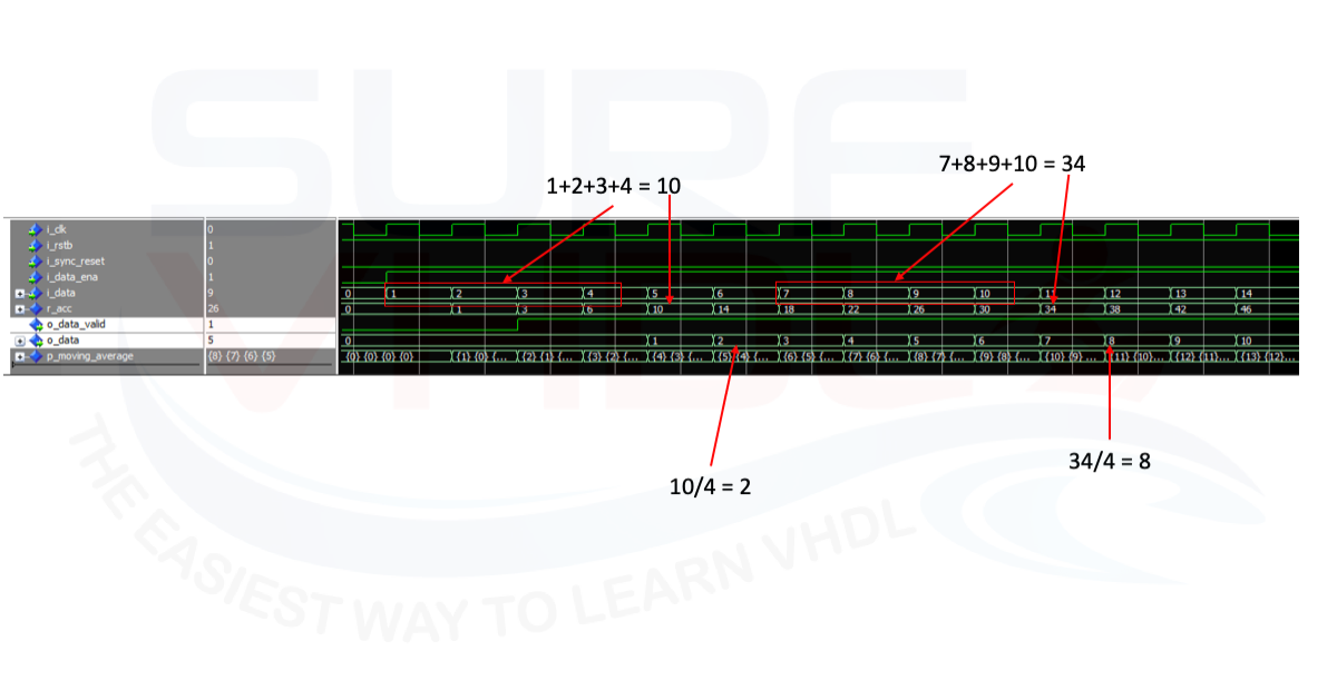
Figure 3 – simulation of moving average on 4 input samples continuous enable
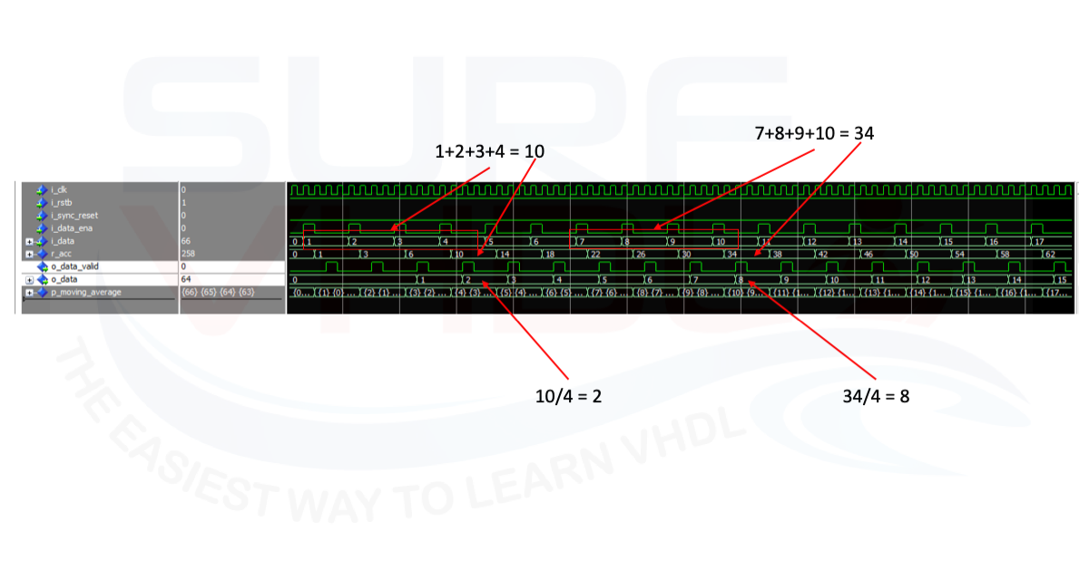
Figure 4 – simulation of moving average on 4 input samples not continuous enable
Both simulations highlight the moving average computing the following:
1+2+3+4 = 10;  => 10/4 = 2

7+8+9+10 = 34; => 34/4 = 8
Conclusion
In this post, we addressed the implementation of a moving average algorithm in VHDL using a very efficient hardware structure that allows the user to implement the moving average using only a data pipe of the dimension of the moving average length and an accumulator.
The control logic is implemented as a synchronous reset that guarantees a correct initial status of the data pipe and accumulator.
In case of very long moving average length, you can adopt the FIFO implementation of the data pipe. The data pipe implemented as a FIFO is treated in this post.
In the case of FIFO implementation, additional control logic must be introduced to handle the initial condition of the FIFO and of the accumulator.
References
[1] Intel FPGA
[2] https://www.mathworks.com/
[3] Scilab