How to implement Galois multiplier in VHDL

Why Galois field

The Galois fields are mainly used in cryptography and error correction algorithms.

If you have never dealt with Galois fields, at the beginning the topic could seem very hard to understand. In this post we want to address the Galois field theory from the practical application point of view.

We will review:

the Galois arithmetic notation, just to understand how to interpret the equation
add/sub operation in Galois field
multiplier in Galois field

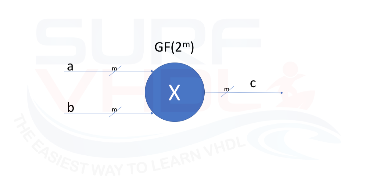
Figure 1 – Galois multiplier in GF(2^m)

The third point is probably the most difficult to understand.

Some readers may find this post frustrating because I will not be very rigorous in the representation of the theory of the Galois fields. This post wishes to give you a practical implementation starting point for your VHDL design using Galois arithmetic.

I have included many references at the bottom of this post that will help you to go deeper in the Galois field theory if you are really interested in it.

For example, Galois fields are at the core of the AES encryption algorithm and Reed-Solomon error correction codes, both widely used in digital communication and storage systems.

Galois field notation

Before starting let’s review some arithmetic notation:

GF(2^m) represents a Galois field of 2^m elements.

A primitive polynomial p(X) is defined to be an irreducible binary polynomial of degree m which divides X^n+1 for n = P^m-1 = 2^m-1 and which does not divide X^i+1 for i<n.

Once a primitive polynomial p(X) is found, then the elements of the Galois field can be generated.

At this link, you can find an example of a primitive polynomial.

Here I don’t want to go deeper in the Galois field theory, so let’s make an example:

p(x) = 1 + x + x^4

This is a primitive polynomial for GF(2^4) = GF(16)

Another primitive polynomial for GF(16) is

p(x) = 1 + x + x^2 + x^3 + x^4

Another notation for p(x) polynomial is the vector representation:

p(x) = x^4 + x + 1 = 10011 = 19dec = 0x13

Addition and Subtraction in GF(2^m)

In GF(2^m) field addition and subtraction are totally equivalent. The addition operation is performed by the XOR operator. In this case, the vector representation of a polynomial is very helpful:

For example, if we want to add two polynomials in GF(16):

G1(x) = x^3 + x^2 +1;
G2(x) = x^3 + x

In vector representation we can write:

G1(x) => 1101
G2(x) => 1010

So G1(x) + G2(x) will be

1101 +
1010 =
------
0111

G1(x)+G2(x) = x^2 + x + 1

Since 2*X^3 = 1 XOR 1 = 0

We obtain the same result for G1(x) – G2(x)

Multiplication in GF(2^m)

In the previous section, we saw that the add/sub operation in the Galois field is very simple since we can perform it as bitwise XOR. The multiplication is a little bit more complicated since the multiplication of two polynomials g(x) and f(x) is defined as follows:

m(x) = (g(x) * f(x)) mod(p(x))

The result of a multiplication is the remainder of the multiplication result f(x)*g(x) divided by the primitive polynomial of the field.

The bitwise multiplication is performed using AND operator.

For example:

f(x) = (a3*x3 + a2*x^2 + a1*x1 + a0)
g(x) = (b3*x3 + b2*x^2 + b1*x1 + b0)

f(x) *g(x) =

(a3*x3 + a2*x^2 + a1*x1 + a0)  * (b3*x3 + b2*x^2 + b1*x1 + b0) =

(b3*x3 + b2*x^2 + b1*x1 + b0) a0 +
(b3*x3 + b2*x^2 + b1*x1 + b0) a1 x^1
(b3*x3 + b2*x^2 + b1*x1 + b0) a2 x^2
(b3*x3 + b2*x^2 + b1*x1 + b0) a3 x^3

As is clear, this is the classical multiplication algorithm where the second row is shifted right by 1, the second by 2 and so on.

The “*” operator is omitted for sake of visualization.

In a practical example:

a3 = 1, a2=0, a1=0, a0 =1 => f(x) = 1001 = 9 dec = 0x9

b3 = 1, b2=1, b1=0, b0= 1 => g(x) = 1101 = 13dec = 0xD


     1101 *
     1001 =
--------------
     1101 + 
    0000  +
   0000   +
  1101    =
--------------
  1100101 = x^6 + x^5 + x^2 + 1 = 101 dec = 0x65

The result does not belong to GF(16) so we need to perform the division by the primitive polynomial.

              x^2 + x
x^4 + x + 1 |_____________________________________________
             x^6 + x^5 +           x^2 +      1
             x^6 +           x^3 + x^2
            --------------------------------------------
             0     x^5 +     x^3 +            1
                   x^5 +           x^2 + x
            --------------------------------------------
                             x^3 + x^2 + x + 1 = 15dec = 0xF

Matlab / Octave example code

a = gf([9],4,19);
b = gf([13],4,19);
m = a*b =15

Interactive Galois Multiplier

Field

Multiplicand A

Multiplier B

Enter decimal values (0–255). Results update automatically.

Implement Multiplier in GF(2^m) using VHDL

The modulo operation in GF(2^m) can be efficiently implemented in hardware using a Linear Feedback Shift Register (LFSR) approach. Each step of the LFSR computes the remainder of a polynomial division, which is exactly what we need for Galois field multiplication.

It is possible to demonstrate that the modulo operation can be implemented using LFSR approach. In this post, you can find an LFSR implementation in VHDL. Here below is reported the VHDL function that implements a Galois multiplier in GF(2^8) using the primitive polynomial

p(x) = 1 + x^2 + x^3 + x^4 + x^8 = 100011101b = 285dec

function mult285 (v1, v2 : in std_logic_vector) return std_logic_vector is
constant m              : integer := 8; 
variable dummy          : std_logic;
variable v_temp         : std_logic_vector(m-1 downto 0);
variable ret            : std_logic_vector(m-1 downto 0);

begin
  v_temp := (others=>'0');   -- 1 + x^2 + x^3 + x^4 + x^8
  for i in 0 to m-1 loop 
    dummy      := v_temp(7);
    v_temp(7 ) := v_temp(6 );
    v_temp(6 ) := v_temp(5 );
    v_temp(5 ) := v_temp(4 );
    v_temp(4 ) := v_temp(3 ) xor dummy;
    v_temp(3 ) := v_temp(2 ) xor dummy;
    v_temp(2 ) := v_temp(1 ) xor dummy;
    v_temp(1 ) := v_temp(0 );
    v_temp(0 ) := dummy;

    for j in 0 to m-1 loop
      v_temp(j) := v_temp(j) xor (v1(j) and v2(m-i-1));
    end loop;
  end loop;
  ret := v_temp;
  return ret;
end mult;

The Matlab / Octave code to verify the result is:

A = gf([34],8,285);
B = gf([55 12 42 231 2 254 1 87],8,285);
C = A.*B

The result is: 192   133   125    98    68    87    34   156

Simulation and Layout of VHDL multiplier in GF(2^8)

Figure 2 shows the VHDL simulation of the mult285 Galois multiplier:

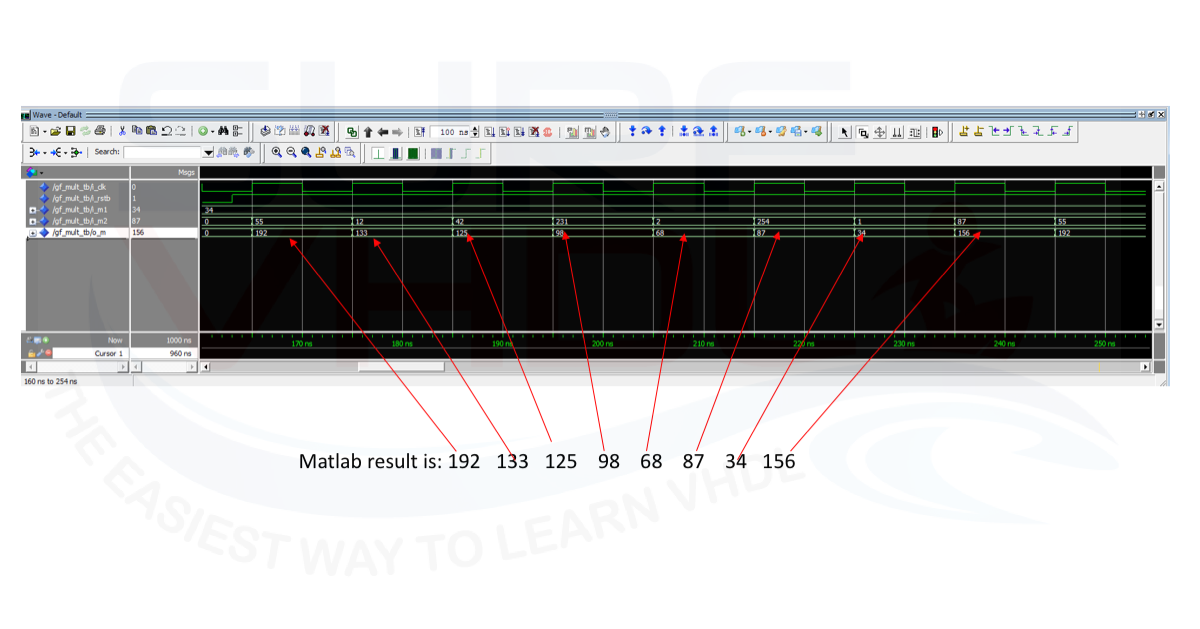
Figure 2 – Modelsim Simulation of VHDL code of Galois multiplier

Figure 3 reports the layout result of the VHDL implementation of the Galois multiplier. In order to evaluate the clock frequency, input and output flip-flops have been added to the VHDL design. The 24 registers reported in the summary are relative to 2×8 = 16 input registers plus 8 output registers. On a Cyclone III FPGA the timing analysis reports 400 MHz

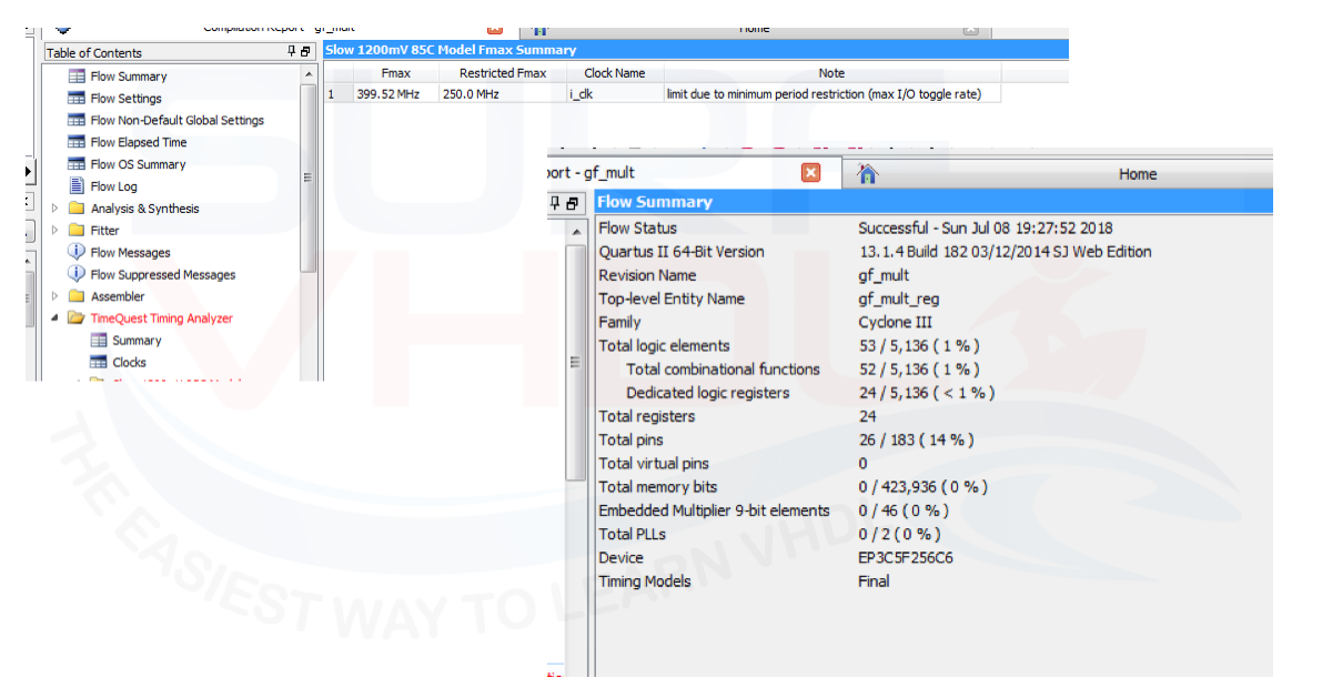
Figure 3 – Layout results of VHDL implementation of Galois multiplier

Conclusion

In this post, we introduced the Galois field arithmetic.

The ADD/SUB operators are reduced to XOR operation, multiplier operation is implemented as XOR and AND operation. The result is reduced using the primitive polynomial relative to the Galois field.

A generic VHDL implementation has been proposed. The VHDL code for the Galois multiplier can be simply modified to perform multiplication operations in different Galois field and different primitive polynomials.